Logical vs. Physical
The logical design is more
conceptual and abstract than the physical design. In the logical design, you
look at the logical relationships among the objects. In the physical design,
you look at the most effective way of storing and retrieving the objects.
Your design should be oriented toward
the needs of the end users. End users typically want to perform analysis and
look at aggregated data, rather than at individual transactions. Your design is
driven primarily by end-user utility, but the end users may not know what they
need until they see it. A well-planned design allows for growth and changes as
the needs of users change and evolve.
Type of Data Modeling?
1) Conceptual Data Model
2) Logical Data Model
3) Physical Data Model
Conceptual
Data Model - Design Step 1
This is First step
for DWH Designing.
Conceptual Data Model is the first step in Data Warehouse design. In conceptual data model, very high level relationships between dimension and fact table is depicted. Conceptual data model not necessarily includes keys, attributes of tables. Conceptual data model gives a very high level idea of proposed Data Warehouse design including possible fact and dimension table. Conceptual data model is the stepping stone to design logical data model of Data Warehouse.
Characteristics of Data Warehouse Conceptual Data Model
1.
It shows only high
level relationship between tables.
2.
It does not show
primary key or column names
3.
It is the stepping
stone of Logical Data Model
Logical
Data Model - Design Step -2
This is Second step
for Designing
Good Logical data model in data warehouse implementation is very important. Logical data model has to be detailed (though some might not agree) as it represents the entire business in one shot and shows relationship between business entities. Logical Model should have following things to make it detailed and self explanatory.
Good Logical data model in data warehouse implementation is very important. Logical data model has to be detailed (though some might not agree) as it represents the entire business in one shot and shows relationship between business entities. Logical Model should have following things to make it detailed and self explanatory.
1.
All entities to be
included in data warehouse
2.
All possible
attributes of each entity
3.
Primary keys of each
entity ( Natural Keys as well as Surrogate Keys )
4.
Relationships between
each every entity
Characteristics of
Data Warehouse Logical Data Model
1.
It has all the
entities which will be used in data warehouse
2.
It shows all possible
attributes of all entities
3.
It depicts the
relationships between all entities
Physical
Data Model - Design Step -3
This is third step
for Designing for DWH Design
Physical Data Model is the actual model which will be created in the database to store the data. It is the most detailed data model in Data Warehouse data modeling. It includes
Physical Data Model is the actual model which will be created in the database to store the data. It is the most detailed data model in Data Warehouse data modeling. It includes
1.
Tables names
2.
All column names of
the table along with data type and size
3.
Primary keys, Foreign
Keys of a table
4.
Constraints
Moving from Logical to Physical Design
In a sense, logical design is what you
draw with a pencil before building your warehouse and physical design is when
you create the database with SQL statements.
Logical models use fully normalized
entities.
The entities are linked together using
relationships.
Attributes are used to describe
the entities.
The UID distinguishes between one
instance of an entity and another.
A graphical way of looking at the
differences between logical and physical designs
Physical Design
Physical design is where you translate
the expected schemas into actual database structures. At this time, you have to
map:
You will have to decide whether to use
a one-to-one mapping as well.
Physical
Design Structures
Translating your schemas into actual
database structures requires creating the following:
Tablespaces
Tablespaces need to be separated by
differences. For example, tables should be separated from their indexes and
small tables should be separated from large tables.
Partitions
Partitioning large tables improves
performance because each partitioned piece is more manageable. Typically, you
partition based on transaction dates in a data warehouse. For example, each
month. This month's worth of data can be assigned its own partition.
Indexes
Data warehouses' indexes resemble OLTP indexes.
An important point is that bitmap indexes are quite common.
Constraints
Constraints are somewhat different in
data warehouses than in OLTP environments because data integrity is reasonably
ensured due to the limited sources of data and because you can check the data
integrity of large files for batch loads. Not null constraints are particularly
common in data warehouses.
Types of Dimensions
in Data Warehousing?
Dimension -
A dimension
table typically has two types of columns, primary keys to fact tables
and textual\descreptive data.?
Fact -A fact table typically has two types of columns, foreign
keys to dimension tables and measures those that contain numeric facts. A fact
table can contain fact’s data on detail or aggregated level.
Types of Dimensions -
Slowly Changing
Dimensions:
Attributes of a dimension that would undergo changes over
time. It depends on the business requirement whether particular attribute
history of changes should be preserved in the data warehouse. This is called a
Slowly Changing Attribute and a dimension containing such an attribute is
called a Slowly Changing Dimension.
Rapidly Changing
Dimensions:
A dimension attribute
that changes frequently is a Rapidly Changing Attribute. If you don’t need to
track the changes, the Rapidly Changing Attribute is no problem, but if you do
need to track the changes, using a standard Slowly Changing Dimension technique
can result in a huge inflation of the size of the dimension. One solution is to
move the attribute to its own dimension, with a separate foreign key in the fact
table. This new dimension is called a Rapidly Changing Dimension.
Junk Dimensions:
A junk dimension is a
single table with a combination of different and unrelated attributes to avoid
having a large number of foreign keys in the fact table. Junk dimensions are
often created to manage the foreign keys created by Rapidly Changing
Dimensions.
Inferred Dimensions:
While loading fact
records, a dimension record may not yet be ready. One solution is to generate
an surrogate key with Null for all the other attributes. This should
technically be called an inferred member, but is often called an inferred
dimension.
Conformed Dimensions:
A Dimension that is
used in multiple locations is called a conformed dimension. A conformed
dimension may be used with multiple fact tables in a single database, or across
multiple data marts or data warehouses.
Degenerate
Dimensions:
A degenerate dimension is when the dimension attribute is
stored as part of fact table, and not in a separate dimension table. These are
essentially dimension keys for which there are no other attributes. In a data
warehouse, these are often used as the result of a drill through query to
analyze the source of an aggregated number in a report. You can use these
values to trace back to transactions in the OLTP system.
Role Playing
Dimensions:
A role-playing
dimension is one where the same dimension key — along with its associated
attributes — can be joined to more than one foreign key in the fact table. For
example, a fact table may include foreign keys for both Ship Date and Delivery
Date. But the same date dimension attributes apply to each foreign key, so you
can join the same dimension table to both foreign keys. Here the date dimension
is taking multiple roles to map ship date as well as delivery date, and hence
the name of Role Playing dimension.
Shrunken Dimensions:
A shrunken dimension
is a subset of another dimension. For example, the Orders fact table may
include a foreign key for Product, but the Target fact table may include a
foreign key only for ProductCategory, which is in the Product table, but much
less granular. Creating a smaller dimension table, with ProductCategory as its
primary key, is one way of dealing with this situation of heterogeneous grain.
If the Product dimension is snowflaked, there is probably already a separate
table for ProductCategory, which can serve as the Shrunken Dimension.
Static Dimensions:
Static dimensions are
not extracted from the original data source, but are created within the context
of the data warehouse. A static dimension can be loaded manually — for example
with Status codes — or it can be generated by a procedure, such as a Date or
Time dimension.
Types of Facts In
Data Warehousing ?
Additive:
Additive facts are
facts that can be summed up through all of the dimensions in the fact table. A
sales fact is a good example for additive fact.
Semi-Additive:
Semi-additive facts
are facts that can be summed up for some of the dimensions in the fact table,
but not the others.
Eg: Daily balances fact can be summed up through the customers dimension but not through the time dimension.
Eg: Daily balances fact can be summed up through the customers dimension but not through the time dimension.
Non-Additive:
Non-additive facts
are facts that cannot be summed up for any of the dimensions present in the
fact table.
Eg: Facts which have percentages, ratios calculated.
Eg: Facts which have percentages, ratios calculated.
Factless Fact Table:
In the real
world, it is possible to have a fact table that contains no measures or facts.
These tables are called “Factless Fact tables”.
Eg: A fact table
which has only product key and date key is a factless fact. There are no
measures in this table. But still you can get the number products sold over a
period of time.
Based on the above
classifications, fact tables are categorized into two:
Cumulative:
This type of fact
table describes what has happened over a period of time. For example, this fact
table may describe the total sales by product by store by day. The facts for this
type of fact tables are mostly additive facts. The first example presented here
is a cumulative fact table.
Snapshot:
This type of fact
table describes the state of things in a particular instance of time, and
usually includes more semi-additive and non-additive facts. The second example
presented here is a snapshot fact table.
Data Warehousing Schemas
A schema is a
collection of database objects, including tables, views, indexes, and synonyms.
There are a variety of ways of arranging schema objects in the schema models
designed for data warehousing. Most data warehouses use a dimensional model.
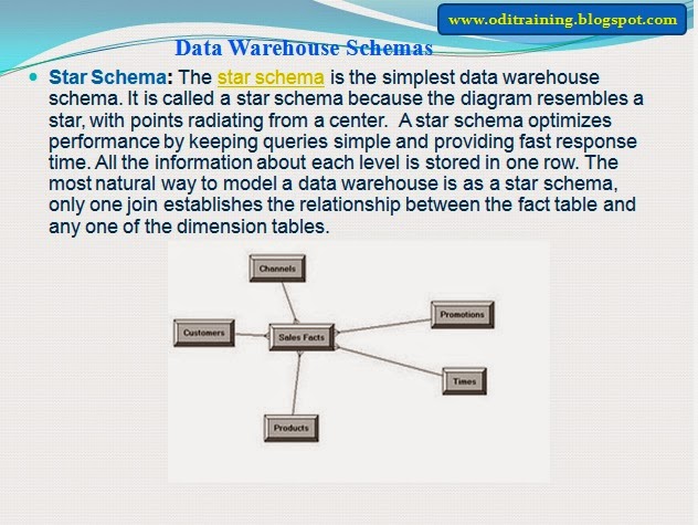
Star Schemas
The star schema
is the simplest data warehouse schema. It is called a star schema because the
diagram of a star schema resembles a star, with points radiating from a center.
The center of the star consists of one or more fact tables and the points of
the star are the dimension tables.

Other Schemas
Some schemas use
third normal form rather than star schemas or the dimensional model.
Snowflake Schema :

Galaxy Schema

Data Warehousing
Objects
The following
types of objects are commonly used in data warehouses:
·
Fact tables are the central tables in your
warehouse schema. Fact tables typically contain facts and foreign keys to the
dimension tables. Fact tables represent data usually numeric and additive that
can be analyzed and examined. Examples include Sales, Cost, and Profit.
·
Dimension tables, also known as lookup or
reference tables, contain the relatively static data in the warehouse. Examples
are stores or products.
Fact Tables
A fact table is
a table in a star schema that contains facts. A fact table typically has two
types of columns: those that contain facts, and those that are foreign keys to
dimension tables. A fact table might contain either detail-level facts or facts
that have been aggregated.
Creating
a New Fact Table
You must define
a fact table for each star schema. A fact table typically has two types of
columns: those that contain facts, and those that are foreign keys to dimension
tables. From a modeling standpoint, the primary key of the fact table is
usually a composite key that is made up of all of its foreign keys;
Dimensions
A dimension is a
structure, often composed of one or more hierarchies, that categorizes data.
Several distinct dimensions, combined with measures, enable you to answer
business questions. Commonly used dimensions are Customer, Product, and Time.
Typical Levels in a Dimension Hierarchy
Dimension data
is typically collected at the lowest level of detail and then aggregated into
higher level totals, which is more useful for analysis. For example, in the
Total_Customer dimension, there are four levels: Total_Customer, Regions,
Territories, and Customers. Data collected at the Customers level is aggregated
to the Territories level. For the Regions dimension, data collected for several
regions such as Western Europe or Eastern Europe might be aggregated as a fact
in the fact table into totals for a larger area such as Europe.
Hierarchies
Hierarchies are
logical structures that use ordered levels as a means of organizing data. A
hierarchy can be used to define data aggregation. For example, in a Time
dimension, a hierarchy might be used to aggregate data from the Month level to
the Quarter level to the Year level. A hierarchy can also be used to define a
navigational drill path and establish a family structure.
Levels
Levels represent
a position in a hierarchy. For example, a Time dimension might have a hierarchy
that represents data at the Month, Quarter, and Year levels. Levels range from
general to very specific, with the root level as the highest, or most general
level. The levels in a dimension are organized into one or more hierarchies.
Level Relationships
Level
relationships specify top-to-bottom ordering of levels from most general (the
root) to most specific information and define the parent-child relationship
between the levels in a hierarchy.
You can define
hierarchies where each level rolls up to the previous level in the dimension or
you can define hierarchies that skip one or multiple levels.
Parallelism and Partitioning
Data warehouses
often contain large tables, and require techniques for both managing these
large tables and providing good query performance across these large tables.
This chapter discusses two key techniques for addressing these needs.
Parallel
execution dramatically reduces response time for data-intensive operations on
large databases typically associated with decision support systems (DSS). You
can also implement parallel execution on certain types of online transaction
processing (OLTP) and hybrid systems.
Overview of Parallel Execution Tuning
Parallel
execution is useful for many types of operations accessing significant amounts
of data. Parallel execution improves processing for:
You can also use parallel execution to access object
types within an Oracle database. For example, you can use parallel execution to
access LOBs (large binary objects).
Parallel
execution benefits systems if they have all of the
following characteristics:
·
Underutilized or intermittently used CPUs (for
example, systems where CPU usage is typically less than 30%)
·
Sufficient memory to support additional
memory-intensive processes such as sorts, hashing, and I/O buffers
When to Implement
Parallel Execution
Parallel
execution provides the greatest performance improvements in decision support
systems (DSS). Online transaction processing (OLTP) systems also benefit from
parallel execution, but usually only during batch processing.
During the day,
most OLTP systems should probably not use parallel execution. During off-hours,
however, parallel execution can effectively process high-volume batch
operations. For example, a bank might use parallelized batch programs to
perform millions of updates to apply interest to accounts..
Tuning Physical Database Layouts
This section
describes how to tune the physical database layout for optimal performance of
parallel execution. The following topics are discussed:
Types of
Parallelism
Different parallel
operations use different types of parallelism. The optimal physical database
layout depends on what parallel operations are most prevalent in your
application.
The basic unit
of parallelism is a called a granule. The
operation being parallelized (a table scan, table update, or index creation,
for example) is divided by Oracle into granules. Parallel execution processes
execute the operation one granule at a time. The number of granules and their
size affect the degree of parallelism (DOP) you can use. It also affects how
well the work is balanced across query server processes.
Block
Range Granules
Block range
granules are the basic unit of most parallel operations. This is true even on
partitioned tables; it is the reason why, on Oracle, the parallel degree is not
related to the number of partitions.
Block range
granules are ranges of physical blocks from a table. Because they are based on
physical data addresses, Oracle can size block range granules to allow better
load balancing. Block range granules permit dynamic parallelism that does not
depend on static preallocation of tables or indexes.
Partition
Granules
When partition
granules are used, a query server process works on an entire partition or
subpartition of a table or index. Because partition granules are statically
determined when a table or index is created, partition granules do not allow as
much flexibility in parallelizing an operation. This means that the allowable
DOP might be limited, and that load might not be well balanced across query
server processes.
Partitioning Data
This section
describes the partitioning features that significantly enhance data access and
greatly improve overall applications performance. This is especially true for
applications accessing tables and indexes with millions of rows and many
gigabytes of data.
Partitioned
tables and indexes facilitate administrative operations by allowing these
operations to work on subsets of data. For example, you can add a new
partition, organize an existing partition, or drop a partition with less than a
second of interruption to a read-only application.
Types
of Partitioning
Oracle offers
three partitioning methods:
Each partitioning method has a different set of
advantages and disadvantages. Thus, each method is appropriate for a particular
situation.
Range Partitioning
Range
partitioning maps data to partitions based on boundaries identified by ranges
of column values that you establish for each partition. This method is often
useful for applications that manage historical data, especially data
warehouses.
Hash Partitioning
Hash
partitioning maps data to partitions based on a hashing algorithm that Oracle
applies to a partitioning key identified by the user. The hashing algorithm
evenly distributes rows among partitions. Therefore, the resulting set of
partitions should be approximately of the same size. This makes hash
partitioning ideal for distributing data evenly across devices. Hash
partitioning is also a good and easy-to-use alternative to range partitioning
when data is not historical in content.
Composite Partitioning
Composite
partitioning combines the features of range and hash partitioning. With
composite partitioning, Oracle first distributes data into partitions according
to boundaries established by the partition ranges. Then Oracle further divides
the data into subpartitions within each range partition. Oracle uses a hashing
algorithm to distribute data into the subpartitions.
Index
Partitioning
You can create
both local and global indexes on a table partitioned by range, hash, or
composite. Local indexes inherit the partitioning attributes of their related
tables. For example, if you create a local index on a composite table, Oracle
automatically partitions the local index using the composite method.
Oracle supports
only range partitioning for global indexes. You cannot partition global indexes
using the hash or composite partitioning methods.
Performance
Issues for Range, Hash, and Composite Partitioning
The following
section describes performance issues for range, hash, and composite
partitioning.
Performance Considerations
for Range Partitioning
Range
partitioning is a convenient method for partitioning historical data. The
boundaries of range partitions define the ordering of the partitions in the
tables or indexes.
In conclusion,
consider using range partitioning when:
·
Very large tables are frequently scanned by a
range predicate on a column that is a good partitioning column, such as
ORDER_DATE or PURCHASE_DATE. Partitioning the table on that column would enable
partitioning pruning.
·
You cannot complete administrative operations on
large tables, such as backup and restore, in an allotted time frame
The following SQL example creates the table Sales for
a period of two years, 1994 and 1995, and partitions it by range according to
the column s_saledate to separate the
data into eight quarters, each corresponding to a partition:
CREATE TABLE sales
(s_productid NUMBER,
s_saledate DATE,
s_custid NUMBER,
s_totalprice NUMBER)
PARTITION BY RANGE(s_saledate)
(PARTITION sal94q1 VALUES LESS THAN TO_DATE (01-APR-1994, DD-MON-YYYY),
PARTITION sal94q2 VALUES LESS THAN TO_DATE (01-JUL-1994, DD-MON-YYYY),
PARTITION sal94q3 VALUES LESS THAN TO_DATE (01-OCT-1994, DD-MON-YYYY),
PARTITION sal94q4 VALUES LESS THAN TO_DATE (01-JAN-1995, DD-MON-YYYY),
PARTITION sal95q1 VALUES LESS THAN TO_DATE (01-APR-1995, DD-MON-YYYY),
PARTITION sal95q2 VALUES LESS THAN TO_DATE (01-JUL-1995, DD-MON-YYYY),
PARTITION sal95q3 VALUES LESS THAN TO_DATE (01-OCT-1995, DD-MON-YYYY),
PARTITION sal95q4 VALUES LESS THAN TO_DATE (01-JAN-1996, DD-MON-YYYY));
Performance
Considerations for Hash Partitioning
Unlike range
partitioning, the way in which Oracle distributes data in hash partitions does
not correspond to a business, or logical, view of the data. Therefore, hash
partitioning is not an effective way to manage historical data. However, hash
partitions share some performance characteristics of range partitions, such as
using partition pruning is limited to equality predicates. You can also use
partition-wise joins, parallel index access and PDML.
As a general
rule, use hash partitioning:
·
To improve the availability and manageability of
large tables or to enable PDML, in tables that do not store historical data
(where range partitioning is not appropriate).
·
To avoid data skew among partitions. Hash
partitioning is an effective means of distributing data, because Oracle hashes
the data into a number of partitions, each of which can reside on a separate
device. Thus, data is evenly spread over as many devices as required to
maximize I/O throughput. Similarly, you can use hash partitioning to evenly
distribute data among the nodes of an MPP platform that uses the Oracle
Parallel Server.
·
If it is important to use partition pruning and
partition-wise joins according to a partitioning key.
The following example creates four
hashed partitions for the table Sales using the column s_productid as the partition
key:
CREATE TABLE sales
(s_productid NUMBER,
s_saledate DATE,
s_custid NUMBER,
s_totalprice NUMBER)
PARTITION BY HASH(s_productid)
PARTITIONS 4;
Specify the
partition names only if you want some of the partitions to have different
properties than the table. Otherwise, Oracle automatically generates internal
names for the partitions. Also, you can use the STORE IN clause to assign
partitions to tablespaces in a round-robin manner.
Performance
Considerations for Composite Partitioning
Composite
partitioning offers the benefits of both range and hash partitioning. With
composite partitioning, Oracle first partitions by range, and then within each
range Oracle creates subpartitions and distributes data within them using a
hashing algorithm. Oracle uses the same hashing algorithm to distribute data
among the hash subpartitions of composite partitioned tables as it does for
hash partitioned tables.
·
Support the use of subpartitions as units of
parallelism for parallel operations such as PDML, for example, space management
and backup and recovery
Using Composite
Partitioning
Use the
composite partitioning method for tables and local indexes if:
·
The contents of a partition may be spread across
multiple tablespaces, devices, or nodes (of an MPP system)
·
You need to use both partition pruning and
partition-wise joins even when the pruning and join predicates use different
columns of the partitioned table
·
You want to use a degree of parallelism that is
greater than the number of partitions for backup, recovery, and parallel
operations
The following
SQL example partitions the table Sales by range on the column s_saledate to create four
partitions. This takes advantage of ordering data by a time frame. Then within
each range partition, the data is further subdivided into four subpartitions by
hash on the column s_productid.
CREATE TABLE sales(
s_productid NUMBER,
s_saledate DATE,
s_custid NUMBER,
s_totalprice)
PARTITION BY RANGE (s_saledate)
SUBPARTITION BY HASH (s_productid) SUBPARTITIONS 4
(PARTITION sal94q1 VALUES LESS THAN TO_DATE (01-APR-1994, DD-MON-YYYY),
PARTITION sal94q2 VALUES LESS THAN TO_DATE (01-JUL-1994, DD-MON-YYYY),
PARTITION sal94q3 VALUES LESS THAN TO_DATE (01-OCT-1994, DD-MON-YYYY),
PARTITION sal94q4 VALUES LESS THAN TO_DATE (01-JAN-1995, DD-MON-YYYY));
Each hashed
subpartition contains sales of a single quarter ordered by product code. The
total number of subpartitions is 16.
Partition Pruning
Partition pruning
is a very important performance feature for data warehouses. In partition
pruning, the cost-based optimizer analyzes FROM and WHERE clauses in SQL
statements to eliminate unneeded partitions when building the partition access
list. This allows Oracle to perform operations only on partitions relevant to
the SQL statement. Oracle does this when you use range, equality, and IN-list
predicates on the range partitioning columns, and equality and IN-list
predicates on the hash partitioning columns.
s_saledate and subpartitioned
by hash on column s_productid,
consider the following SQL statement:
SELECT * FROM sales
WHERE s_saledate BETWEEN TO_DATE(01-JUL-1994, DD-MON-YYYY) AND
TO_DATE(01-OCT-1994, DD-MON-YYYY) AND s_productid = 1200;
Oracle uses the
predicate on the partitioning columns to perform partition pruning as follows:
·
When using hash partitioning, Oracle accesses
only the third partition, h3, where rows with s_productid equal
to 1200 are mapped
Pruning
Using DATE Columns
In the previous
example, the date value was fully specified, 4 digits for year, using the
TO_DATE function. While this is the recommended format for specifying date
values, the optimizer can prune partitions using the predicates on s_saledate when you use other
formats, as in the following examples:
SELECT * FROM sales
WHERE s_saledate BETWEEN TO_DATE(01-JUL-1994, DD-MON-YY) AND
TO_DATE(01-OCT-1994, DD-MON-YY) AND s_productid = 1200;
SELECT * FROM sales
WHERE s_saledate BETWEEN '01-JUL-1994' AND
'01-OCT-1994' AND s_productid = 1200;
However, you
will not be able to see which partitions Oracle is accessing as is usually
shown on the partition_start and partition_stop columns of the
EXPLAIN PLAN command output on the SQL statement. Instead, you will see the
keyword 'KEY' for both columns.
Avoiding
I/O Bottlenecks
To avoid I/O
bottlenecks, when Oracle is not scanning all partitions because some have been
eliminated by pruning, spread each partition over several devices. On MPP
systems, spread those devices over multiple nodes.
Partition-wise
Joins
Partition-wise
joins reduce query response time by minimizing the amount of data exchanged
among query servers when joins execute in parallel. This significantly reduces
response time and resource utilization, both in terms of CPU and memory. In
Oracle Parallel Server (OPS) environments, it also avoids or at least limits the
data traffic over the interconnect, which is the key to achieving good
scalability for massive join operations.
There are two
variations of partition-wise join, full and partial, as discussed under the
following headings.
Full
Partition-wise Joins
A full
partition-wise join divides a large join into smaller joins between a pair of
partitions from the two joined tables. To use this feature, you must
equi-partition both tables on their join keys. For example, consider a large
join between a sales table and a customer table on the column customerid. The query "find
the records of all customers who bought more than 100 articles in Quarter 3 of
1994" is a typical example of a SQL statement performing such a join. The
following is an example of this:
SELECT c_customer_name, COUNT(*)
FROM sales, customer
WHERE s_customerid = c_customerid
AND s_saledate BETWEEN TO_DATE(01-jul-1994, DD-MON-YYYY) AND
TO_DATE(01-oct-1994, DD-MON-YYYY)
GROUP BY c_customer_name HAVING
COUNT(*) > 100;
This is a very
large join typical in data warehousing environments. The entire customer table
is joined with one quarter of the sales data. In large data warehouse
applications, it might mean joining millions of rows. The join method to use in
that case is obviously a hash join. But you can reduce the processing time for
this hash join even more if both tables are equi-partitioned on the customerid column. This
enables a full partition-wise join.
Hash - Hash
This is the
simplest method: the Customer and Sales tables are both partitioned by hash
into 16 partitions, on s_customerid and c_customerid respectively.
This partitioning method should enable full partition-wise join when the tables
are joined on the customerid column.
In serial, this
join is performed between a pair of matching hash partitions at a time: when
one partition pair has been joined, the join of another partition pair begins.
The join completes when the 16 partition pairs have been processed.
Comments
Post a Comment